


RISA-3D v13 includes a new Ritz Vector Solver for the Dynamic analysis. When running a Response Spectrum analysis for seismic design, some structures experience large numbers of local modes that don’t contribute to the lateral response of the structure. The use of load-dependent Ritz vectors (rather than true mode shapes) can greatly improve the speed and accuracy of a Response Spectra analysis for these types of models.
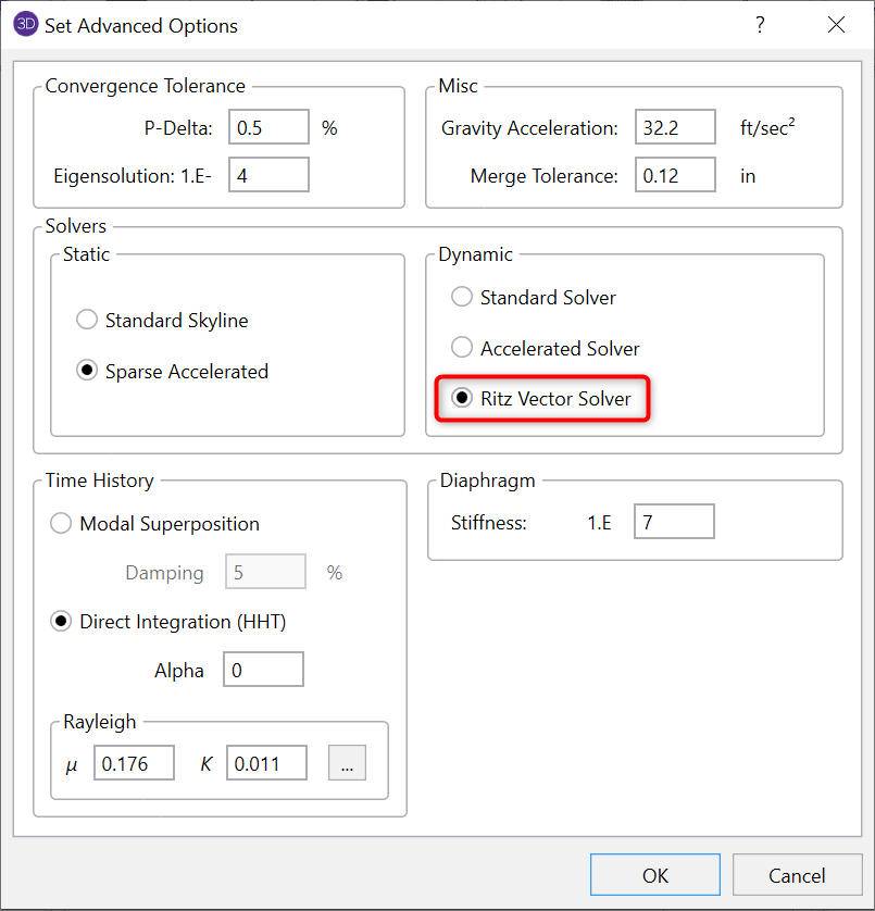
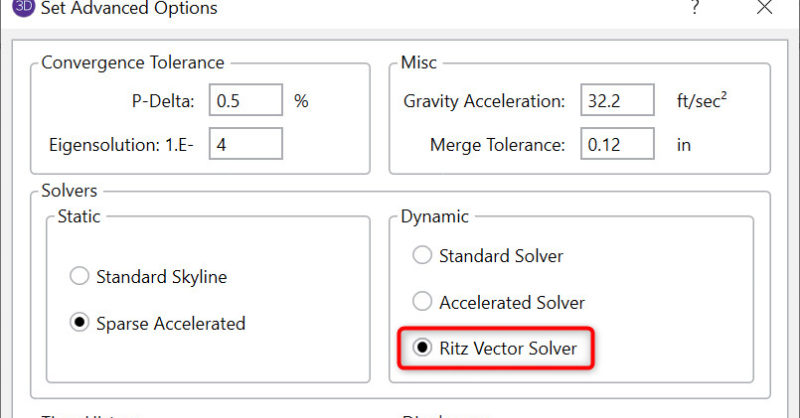
There is a new option added to the Dynamic solution options as shown to the right. This dialog can be found by clicking on the Advanced button from the Solution tab of the Model Settings.
RISA-3D Output
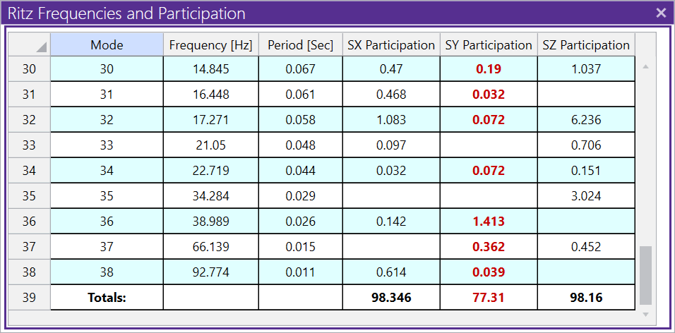
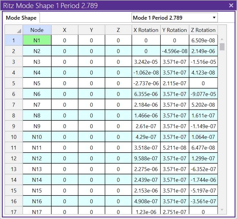
In general, the Ritz vectors will be very similar in shape and frequency to the true dynamic results, though they are not expected to be identical. For that reason, the RISA-3D results will identify them as Ritz Vectors (rather than Mode Shapes) and Ritz Frequencies in the title bar of the dynamic results spreadsheets.
Simplified Overview
The general concept is that a static solution in the direction of the seismic loading will form a good basis for the approximate mode shapes of the structure which then leads to natural frequency calculations.
This concept is nothing new. The Rayleigh-Ritz method for natural period calculations have been used for many, many years as an excellent hand calculation method for estimating the first fundamental period. That method results in ASCE 7’s natural period equation 15.4-6:
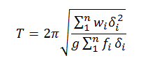
This equation uses the mass distribution at each floor (wi), the static displacement of that floor (δi), and the lateral force applied to that floor (fi) to come up with a fairly accurate estimate of the natural period. Ritz vectors can be viewed as an extension of this concept where additional modes are calculated based on assumed modal forces derived from the previous mode shape / Ritz vector.
It should be noted that the force vector used in this method does not need to closely match the seismic force distribution for the first mode. A very approximate force vector (like a wind load vector or structure weight applied laterally) works as well.
Practical Advantages of Ritz Vectors
The use of Ritz vectors in a Response Spectra or Time-History analysis offers a number of practical advantages over traditional mode shapes.
-
Ritz vectors will ignore modes that do not contribute to the response of the structure in the direction of interest. Therefore, Ritz vectors require fewer modes to get to 90% mass participation.
-
Ritz vectors automatically account for the residual rigid response of the structure.
-
A Ritz vector solution is faster and requires less memory than a dynamic analysis using traditional eigen modes.
Limitations with Ritz Vectors
-
Ritz vectors will closely resemble actual mode shapes, especially for the first few modes. However, they are not true eigenmodes.
-
When mass participation is low, the residual response can occur at frequency lower than the actual rigid response, thereby resulting in lower spectral forces in the Response Spectra analysis.
The (Painfully) Technical Details
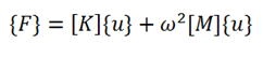
It’s best to start with the basic dynamic equilibrium equation shown below. This has a dynamic component based on the mass matrix (ω2*[M]*{u}) and a displacement component based on the stiffness matrix ([K]*{u}).
The first Ritz vector is calculated as the static displacement vector of the structure when it is subject to some initial force vector. This means the mass term from the equation above is ignored. The above equation then simplifies down to the simpler equation, F = [K] {uo}. where {uo} is the basis for the first Ritz vector / mode shape. This solution {uo} is then mass normalized to take a form closer to a true eigen mode {Φo}.
In RISA-3D, the initial force vector is based on the load combination used in the definition of dynamic mass with the load being applied only in the direction of the desired seismic response. This is done automatically without requiring the users to derive their own force for each direction.
Since the shape of that first displacement vector is purely static in nature ({uo} from the equation F = [K] {uo}), the error in the estimate of the dynamic force can be represented as being proportional to the mass matrix times the first mode ({uo} or {Φo}).
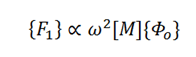
The second mode can then be solved for. Higher order modes are then approximated using the same general concept, by estimating the dynamic force as being proportional to the mass matrix times the previous mode shape.
The procedure can be viewed in more detail in Chapter 14 of “Three Dimensional Static and Dynamic Analysis of Structures” by Ed Wilson. Specifically, section 14.8 (Generation of Load-Dependent Ritz Vectors).
Using this procedure, it is clear that the modes found should only be modes that produce displacement in the desired directions.