Solution

Note:

• The linear-elastic behavior of the program implicitly means that non-linear (2nd order) behavior is not generally supported. Tension-structures such as guy cables or fabric structures would fall into this non-linear category. Please see the Modeling Tips section for some ways to approximate this behavior. This note applies to all elements in the program (wall panels, plates, members, etc.).

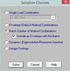
Four solution options are presented when you click Solve on the menu. Some of the options require other solution types to be performed. See Results for information on solution results. For additional information on Dynamic Analysis and Response Spectra Analysis results refer directly to those sections. For footing design within RISA-3D or RISA-2D see the Footing Design topic. For connection design within RISA-3D see the RISAConnection Integration topic.

What do you want to do?

• Perform a dynamic analysis.
• Perform a response spectra analysis.
• Perform a Time History solution.
• Perform a Static Solution

What do you want to know?

• What is an Envelope Solution?
• What is an Batch  Solution?

Static Solutions / Stiffness Matrix

Static solutions are based on load combinations and may be performed on any defined load combinations. When a static solution has been performed and the results are available the "S" icon on the status bar in the lower left corner will change from  to . If any changes are made to the model that invalidate the results then the results will be cleared and another solution will be necessary.

The solution is based on the widely accepted linear elastic stiffness method for solution of the model.  The stiffness of each element of the structure is calculated independently.  These element stiffnesses are then combined to produce the model's overall (global) stiffness matrix. This global matrix is then solved versus the applied loads to calculate joint deflections. These joint deflections are then used to calculate the individual element stresses. The primary reference for the procedures used is Finite Element Procedures, by K. J. Bathe (Prentice-Hall, 1996).

Skyline Solver 

This solution method is also sometimes referred to as an Active Column solution method. In finite element analysis, the nonzero terms of the stiffness matrix are always clustered around the main diagonal of the stiffness matrix. Therefore, the Skyline or Active Column solutions take advantage of this by condensing the stiffness matrix to exclude any zero stiffness terms that exist beyond the last non-zero term in that column of the matrix.

Since the majority of terms in a stiffness matrix are zero stiffness terms, this method greatly reduces the storage requirements needed to store the full stiffness matrix. However, for large models (+10,000 joints) , the memory requirements even for a skyline solution can be problematic.

This solution method has been used successfully in RISA for more than 20 years, and has proven its accuracy continuously during that time.

Single Combination Solutions

Choose this option to solve one load combination by itself.

Envelope Solutions

Static solutions may also be performed on multiple combinations and the results enveloped to show only the minimum and maximum results. Each of the results spreadsheets will contain minimum and maximum values for each result and also the corresponding load combination. The member detail report and deflected shape plots are not available for envelope solutions. See Load Combinations to learn how to mark combinations for an envelope solution.

Batch Solutions

Static solutions may be performed on multiple combinations and the results retained for each solution. When performing a batch solution, you have the option to also include a set of envelope results. This is useful when an envelope result is desired to quickly determine a controlling load combination, but when the investigation of that load combination required the greater details given with batch solution results. When using the Batch + Envelope Solution, to view the envelope results, click on a spreadsheet in the Results toolbar. To view the batch results, click on that same spreadsheet in the Results toolbar a second time. Both the envelope and batch solution spreadsheets should now be available simultaneously.

You may group the results by item or by load combination by choosing from the Results Presentation options on the Results Menu. For example you can have all the combination results for member M1 together or you can have all the member results for Load Combination "D+L" together. See Load Combinations to learn how to mark combinations for a batch solution.

Dynamic Solutions - Eigenvalues & Mode Shapes

In this section, the term "Dynamic Solutions" refers to solving of the dynamic properties of a structure. This involves assembling the mass matrix, solving for the eigen values (natural periods / frequencies), as well as determining the mode shapes of vibration associated with each period / frequency. Dynamic analysis requires a load combination, but this combination is merely used to determine the mass of the model. See Dynamic (Modal) Analysis for much more information.

When a dynamic solution has been performed and the results are available the "D" icon on the status bar in the lower left corner will change from  to . If any changes are made to the mode that invalidates the results then the results will be cleared and another solution is necessary.

Accelerated Solver 

The Accelerated Solver is actually three solvers in one: A Direct Jacobian, an Accelerated Sub-Space solver, and a Lanczos Solver. Each of these solvers will have a certain range of models for which it is most efficient. Therefore, RISA will automatically detect which should be most efficient for the given model and use that solver for the eigen-solution. This solver is much more efficient than the standard solver and will fine frequencies and mode shapes in a fraction of the time the standard solver. Therefore, it is the default solution option.

Standard Solver 

This solver uses sub-space iteration to solve for the Eigen values. This solver has been used for years and the accuracy of the results is very well established. It has been included mostly for comparative / verification purposes.

Ritz Vector Solver 

This solver uses Load Dependent Ritz (LDR) vectors to bias the dynamic solution. This means that the solution does not necessarily represent the true mode shapes or natural frequencies of the structure. As such, this solution should not be used in cases where the natural frequencies and modes shapes are the main goal.

Ritz vectors are derived by using a static displacement vector as the basis of the derived vector, only allowing for the solution of modes / vectors that will be excited by the initial loading or which will contribute to the total response. In RISA, the initial static displacement vectors are based on the load combination used for the definition of dynamic mass. The mass defined in this load combination is converted into a static load in each direction for which a Response Spectra solution is requested. The solution of which forms the basis for the initial Ritz Vectors.

Note:

• For cases where the mode shapes and frequencies are used to estimate dynamic response (i.e. Response Spectra or Time History analysis), it has been demonstrated that using Ritz vectors can produce a more accurate response than would be obtained using the same number of true eigen modes.
• It is possible, however, for there to be some frequency shift in the mass participation. For the case of earthquake response of a typical building structure, this frequency shift should result in a more conservative base shear than would be produced by a true eigen solution producing the same amount of mass participation.
• In particular Ritz Vectors are useful for cases in which it is difficult to obtain the desired level of mass participation with a traditional eigen value analysis. This is because Ritz vectors are biased towards a presumed deflected shape.
• When Ritz Vectors are used for a Time History analysis the LC used as the basis for the dynamic mass should contain TH loading at the main joints of the structure. The program will detect this and then include the Time History Load function in the initial static displacement vector. This doesn't change the mass matrix at all. But, it will bias the Ritz Vectors to displacements at those joints which leads to a more accurate Time History response with fewer modes.

Dynamic Solutions - Response Spectra

• Whenever a dynamic / eigen solution has been performed the "D" icon on the status bar in the lower left corner will change from  to .
• If any changes are made to the model that invalidate these dynamic results (even if they don't invalidate the mass matrix), the dynamic results will be cleared and need to be re-solved before a time history analysis can be performed.

Note:

• Alpha will default to zero, at which point the solution is identical to the Newmark Beta method using integration constants Beta = 0.25 and gamma = 0.5.
• A negative value for alpha is often used then the desire is to dissipate energy associated with higher frequency response. This makes the HHT solution methodology more stable than other solution methods, and may allow the user to set their integration time step slightly larger to improve time history solution speed. Refer to topic Dynamic Analysis - Time History for more information on setting time steps.
• RISA requires an Eigensolution or Ritz Vector solution even when Direct Integration is used. Refer to Required Number of Modes for a discussion on this topic.