
This section summarizes the theoretical formulation and the implementation of P-Delta analysis using ADAPT’s FRAME finite element solver.
P-Delta analysis is a methodology to compute structures which are prone to the load-displacement interaction, resulting in second-order effects. This basically means that the load which is applied to the structure is parametrically controlling the elastic or inelastic response of the structure. Such structures cannot be solved using standard (single step) linear elastic process [KS]*[D]=[F], but instead requires the iterative approach.
There are two types of P-Delta methodologies:
Large P-Delta (P-Δ)
Small P-delta (P-δ)
“Large” P-Delta (P-Δ) refers to the second order effect associated with the lateral translation of the members. The idea of large P-Delta (P-Δ) is illustrated in the following image.
Click on image to enlarge
“Small” P-delta (P-δ) refers to the second order effect associated with the member curvature. The idea of small P-delta (P-δ) is illustrated in the following image.

Click on image to enlarge
The difference between these two methodologies lies in the mathematical formulation as well as in finite element solution approach. On the level of mathematical formulation (which translates into finite element formulation) the difference can come from excluding or including higher order terms (geometric non linearity).
On the level of a finite element (FE) solution, the difference between these two methodologies will also depend on the granularity of meshing as well as prescribed number of iterations. For refined meshes, the solutions using both approaches may lead to similar solutions.
The most accurate methodology is when nonlinear 2nd-order FE analysis is used. In such cases, the effects of member curvature are covered by high order formulation (geometric non linearity), and for this reason it is a (small) P-delta solution.
Linear elastic 2nd order analysis is commonly used in engineering practice and allowed by design codes (e.g. ACI 318). Linear elastic 2nd order analysis, which is based on a geometric stiffness matrix, is considered sufficiently accurate for engineering applications.
The implementation focus in ADAPT-Builder’s FRAME solver is that of P-Delta (P-Δ) 2nd-order, linear elastic, and small displacements calculations in conjunction with the geometric stiffness matrix of a frame (beam/column) element.
A geometric stiffness matrix, KG, accounts for the effect of loads existing in the element on the stiffness of the element. For example, it is well known that the axial load in a beam-column has an appreciable effect on the lateral stiffness. The geometric stiffness matrix KG is an adjustment to the conventional elastic stiffness matrix to account for such effects.
The adjusted (combined) stiffness matrix of the entire system is used in the course of finite element computation, to obtain a solution which incorporates the effects of load on the stiffness of the system. Such computational process requires iterative, or a pseudo-iterative, approach in order to converge to a solution for which the adjusted (combined) stiffness matrix corresponds well to the applied loads, and the displacements for two consecutive iterations are within prescribed tolerance.
The geometric stiffness matrix can be derived for frame (beam and column) elements as well as for plate shell elements. The derivation of the geometric stiffness matrix for frame elements is relatively simple and straight-forward.
The derivation of geometric stiffness for plate triangular and quadrilateral elements is much more complex, and it presents multiple mathematical and numerical challenges. The current implementation in ADAPT-Builder’s frame solver does not cover the geometric stiffness of plate shell element.
The focus for the current implementation is on the geometric stiffness of a frame element, since it plays a prominent role when computing structures supported on columns, such as unbraced or partially braced multi-level frames and buildings.
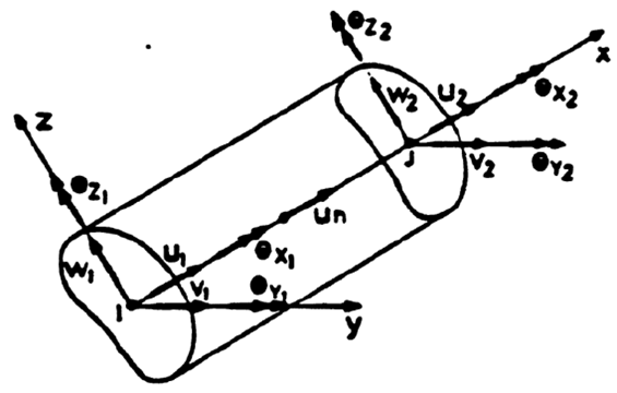
A standard 3-dimensional (Bernoulli-Euler) frame element is assumed, having the following local coordinate system:
Click on image to enlarge
The elastic stiffness matrix of such a 3-dimensional frame element in the local coordinate system can be represented by the following 12x12 matrix:

Click on image to enlarge
The corresponding geometric stiffness matrix of a 3-dimensional frame element in the local coordinate system can be represented by the following 12x12 matrix:

Click on image to enlarge
Where:
P – axial force in the element.
L – length of the element.
Iρ – Ix+Iy – Polar moment of inertia.
The combined elastic geometric stiffness matrix of frame elements as implemented in ADAPT’s FRAME solver can be represented by the sum of each matrix location entry from the matrices shown above.
The combined elastic and geometric stiffness matrices [Ke+Kg] of individual frame elements are transformed from the local to global coordinate system and assembled into a stiffness matrix of the entire system [Ks]. The results are obtained in a similar fashion by solving the system of finite element equations:
[Ks]*[D]=[F]
Where:
[D] – nodal displacement vector (unknown)
[F] – nodal force (load) vector.
Because geometric matrices [Kg] are parametrized by the axial forces acting in the elements, the solution needs to be calculated iteratively, and the elements of geometric matrices updated for each iteration. In the first iteration, the system is solved as a regular elastic model, without use of the geometric stiffness matrices. In the subsequent solutions, geometric matrices are employed. Typically, iterative processing converges quickly, especially when analyzing multi-level structures, where the magnitude of axial forces in the elements does not change significantly from one iteration to the other. For practical purposes, two or three iterations are sufficient to obtain a relevant solution.
Because P-Delta analysis is a pseudo-nonlinear process, the solutions should normally be obtained using complete load combinations instead of individual load cases since the solutions cannot be linearly combined. This causes the amount of time needed to obtain the solutions for multiple combinations to be more significant and computationally consumptive than when solving individual load cases.
In typical engineering practice, P-Delta analysis is employed in conjunction with lateral analysis, when wind or earthquake loads are acting. The purpose is to capture the amplification of the lateral effects due to P-Delta effects. For such cases, literature suggests that simplifications are possible in the process, so as to limit the computation time. For example, when the following load combination is involved:
U=1.2D + 1.0L + 0.2S + 1.0E
there are typically several variations of it because the seismic load can be acting in a few different ways. Literature sources suggest that the amplification of lateral loads due to P-Delta effects may, in such situations, be obtained by evaluating the geometric stiffness matrices based on the vertical and sustained gravity components of the load combination such as:
U=1.2D + 1.0L + 0.2S
The assumption here is that the lateral loads have negligible effect on axial forces in vertical elements (columns). Under this assumption several combinations of the same type can be solved in parallel using the same iteration process. The first “master” load case (or vertical combination) may be solved, such as:
U=1.2D + 1.0L + 0.2S
This combination is used to evaluate the geometric matrices. The remaining combinations, such as all the lateral variations of:
U=1.2D + 1.0L + 0.2S + 1.0E
can be solved in parallel using the same set of system matrices. This performance improvement is implemented in FRAME as part of batch solutions as described later in the document.
There is limited information with regards to how prestressing or post-tensioning forces are to be handled when performing P-Delta analysis. The comments contained in this section are, for the most part, the opinion of ADAPT and may not be in agreement with other literature sources.
Prestressing is a source of compressive axial forces in the elements. Prestressing and post-tensioning tendons are embedded inside the element (if not external); therefore, eccentricity of the tendon remains unchanged with regards to the deformed section. Subsequently there is no amplification effect for the tendon’s transverse actions as a result of the compressive prestressing force. Similarly, there is no amplification effect when a prestressing force acts in conjunction with transverse loads different than PT. An embedded tendon itself is not a source of buckling (secondary) effect for the host concrete element.
For this reason, it is unnecessary to account for the axial force due to prestressing when evaluating the elements of the geometric stiffness matrices. The axial forces to be used for evaluating the geometric stiffness matrices should primarily be based on gravity load components. The transverse effects of the post-tensioning (“load balancing” effects) may interact with the axial forces in the elements due to external loads, such as gravity loads, leading to the secondary (P-Delta) effects. In other words, the P-Delta effects are possible when tendon exerts transverse load on the element in conjunction with external (non-PT) axial force within the element. The reason for this is that post-tensioning generates the deformation of the member, therefore an additional external axial force acting on the member may lead to the amplification of the deformation caused by the tendon.
Let us assume that we have the following load combination to be analyzed for P-Delta:
U=1.2D + 1.0L + 0.2S + 1.0P + 1.0E
Based on what was written before in this section, two load cases in this combination, prestressing “P” and lateral “E”, are the obvious candidates to be excluded from evaluation of the geometric stiffness matrices.
The implementation of P-Delta in ADAPT-Builder’s FRAME solver automatically excludes the contribution of prestressing force from the calculation of the geometric stiffness matrix. This takes place for all possible arrangements of load cases (load combinations) in the INP input file, both in singular and batch processing modes.
ADAPT-Builder’s frame solver has the capability to solve multiple load cases in single solution handling (using the same system stiffness matrix). In such a case, the right-hand side of the FEM equation system consists of multiple nodal load vectors, and the solution consists of multiple vectors of nodal displacements. Normally these types of solutions are only possible for linear analysis. The advantage of this feature is a significant reduction of the computation time, because the system stiffness matrix needs to be solved only once for multiple load combinations.
Since P-Delta is pseudo nonlinear, it is not possible to obtain fully accurate P-Delta solutions when using load batches. When analysis is performed using load batches, the first load set (partial combination) from the batch will be used to evaluate the combined stiffness matrix of the system [Ke+Kg], while the remaining load sets in the batch may include the load components which are negligible or inappropriate for calculation of the geometric stiffness.
For the load combination mentioned above, the first load set (partial combination, or “master” combination) to be used for evaluating the combined stiffness matrix of the system [Ke+Kg] will be as follows:
U=1.2D + 1.0L + 0.2S + 1.0P
In the above combination, the prestressing component will be ignored by the program when evaluating geometric stiffness matrices, but will be considered otherwise.
The remaining load sets for a given load batch may represent the complete combinations such as:
U=1.2D + 1.0L + 0.2S + 1.0P + 1.0E
Typically, there are several variations of the lateral load “E” (or similarly, “W” for wind), therefore the load batch will produce several solutions using a single system matrix [Ke+Kg], if those variations are included as combinations.
Similar multi-load solutions can be obtained when the lateral load is of wind type.
The usage of batch loads required additional provisions in ADAPT-Builder’s GUI, in order to automate the process of generation of INP input file. The algorithm developed in the GUI allows for combinations to be set to the ‘P-Delta” analysis/design option type. This algorithm performs the following functions:
Load Combinations will be internally sorted according to:
Combination category (SLS, ULS etc)
Type of analysis (P-DELTA included or excluded)
Combination factors for each load component (SW, DL, SDL, LL, PT, EQ, etc.)
Load combinations which are selected for P-Delta analysis will be assigned into groups (batches) based on identical load factors for vertical (gravity) load cases.
The group (batch) which will be solved together needs to have all load components and factors identical, except for the lateral component.
For each P-Delta load combination batch, the algorithm creates a master combination which includes identical load components. This master load combination is used to establish the geometric matrix.
The algorithm for P-Delta load combination post-processing has the ability to switch from batch load solutions to individual solutions. Although the load batch approach is oftentimes sufficiently accurate when analyzing multistory buildings with prevailing gravity loads, it may sometimes be insufficient. The program gives you an option to switch from batch load solutions to individual solutions.
Individual solutions may be computationally more consuming, but sometimes can be useful for the engineer. The use of individual solutions is especially justified when the structural model is fully developed and requires final results.
If P-Delta load combinations are developed such that there is no unique set of load cases and factors that is repeated, each combination is solved independently with a unique geometric matrix, not shared.
In ADAPT-Builder’s solver, the computations using P-Delta methodology can only be performed for frame (building) structures. Currently the FRAME solver does not support P-Delta computations for models which are supported on uni-directional (compression only) springs. The use of uni-directional springs requires an iterative (pseudo-nonlinear) solution, which would be in conflict with the iteration process for P-Delta analysis as currently implemented. ADAPT-Builder’s GUI performs a check for uni-directional springs, and if present, disables the option to run P-Delta analysis. In particular, P-Delta analysis is disabled when analyzing models in MAT or SOG modes of the program.
The FEM analysis which includes geometric stiffness matrices may, on occasion, result in non-solvable models. This is possible when the magnitude of the axial loads in the columns is close to or above the critical buckling loads. Even if for a single column, the value of axial load exceeds critical, the resulting combined stiffness matrix [Ke+Kg] of this element may be singular and unsolvable. It is advisable that an engineer should perform preliminary static (non-P-delta) analysis first, in order to evaluate the magnitude of axial forces in columns, to make sure their critical loads are not exceeded. Graphical reporting of amplification factors for both moment and drift are available for P-delta load combinations.
ACI-318 code defines the requirements for structural analysis of concrete member design and permits the 1st order analysis with moment magnification, and/or, elastic second 2nd-order analysis. Other methods included are inelastic 2nd-order and non-linear FEM.
Stability Limit
Starting from the 2008 edition of ACI 318 code, a unified stability requirement was introduced on compressive members (primarily columns) which limits the moment amplification due to P-Delta to 1.4 as a ratio of 2nd/1st order moments. This provision was presented in this edition of the code as follows:

Click on image to enlarge
When a structural model satisfies this requirement for each of its columns, its stability is is assured both globally and locally.
The functionality for P-Delta analysis inside ADAPT-Builder’s FRAME solver includes new procedures for calculation of the following amplification factors:
MAF – moment amplification factors at the ends of frame elements.
DAF – drift amplification factors.
These values are stored in ADO output files for P-Delta solutions and are used as the source files for producing both graphical and XLS outputs for moment, drift, and displacements.
In the previous editions of the ACI code, the basic measure of stability was based on the so-called “stability index.” ADAPT-Builder’s FRAME solver does not support this particular calculation and stability is reported in the aforementioned method.
Section Stiffness Reduction
The 2008 edition of the ACI 318 code sets forth the following requirements regarding elastic 2nd-order P-Delta analysis:

Click on image to enlarge
In lieu of more precise determination of the properties of cracked sections, the following simplified stiffness reductions are permissible:

Click on image to enlarge
The above stiffness reductions are primary prescribed for nonprestressed members. For prestressed members ACI 318 states the following:
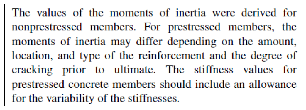
Click on image to enlarge
Assuming that structural floors and beams are prestressed, the reductions of stiffness included in section 10.10.4.1 are at least applicable to columns and walls. This means that PT structural models should, at the very minimum, be executed using flexural stiffness reduction factors equal to 0.7 for all vertical support elements (columns and walls). In case it is hard to determine the state cracking in structural walls, the more appropriate flexural stiffness reduction factor equals 0.35.
ADAPT-Builder allows users to define ‘Usage Cases’ to set modifiers for the structural components. A user is able to define, store, and obtain solutions for various usage cases. Refer to the Stiffness Modifiers & Usage Case topic of this help file for additional information regarding Usage Cases and Stiffness Modifiers.
Eurocode 2 Section 5.8.2 states that global 2nd-order effects may be ignored if they are less than 10% of the first order effects. As an alternative, if the slenderness (l) is less than the slenderness limit (llim), then second order effects may be ignored. The main provision for this is as follows:

Click on image to enlarge
Essentially, this is a definition of a threshold between a non-sway and sway structure. The above limitation frees an engineer from more detailed slenderness design. The most adequate verification of this criterion can be obtained as a result of 2nd-order P-Delta analysis. In case the 10% limits for standard analysis are exceeded and second order analysis is needed, Eurocode 2 specifies the following general requirements:

Click on image to enlarge
This practically stipulates that when analysis is based on assumption of linear materials and geometric non-linearity, the reduced stiffness approach needs to be taken, similarly to the requirements of ACI code. Even though the detailed requirements may be different, the general ideas are similar in nature. From the standpoint of implementation in ADAPT-Builder’s FRAME solver, the most interesting aspect is employing the use of usage cases with defined stiffness modifiers following code recommendations.
Eurocode 2 presents the provisions for 2nd-order analysis of individual isolated members and for entire structures (global analysis). With regards to the calculations performed by ADAPT-Builder’s frame solver, provisions for isolated members are of no particular interest. The provisions for global analysis are of importance here.
Eurocode 2 mentions the following methods of analysis of slenderness effects:

Click on image to enlarge
The general method is based on non-linear analysis, including geometric non-linearity i.e. second order effects. The provisions for general method (5.8.6) stipulate that both material and geometrical non-linearity should be used. In case software does not handle material non-linearity, these effects need to be accounted for by means of stiffness reductions, as was mentioned before, and should be based on the required nominal stiffness method of section 5.8.7. The nominal stiffness method is primarily meant for global analysis. The nominal curvature method (5.8.8) is primarily to be used for isolated members, and therefore it is not useful in application within ADAPT-Builder.
The nominal stiffness method (5.8.7) presents the following requirements regarding calculations of stiffness reductions of slender elements:

Click on image to enlarge

Click on image to enlarge

Click on image to enlarge

Click on image to enlarge
The provisions of 5.8.7(4) are the most relevant from the standpoint of the implementation of P-Delta in ADAPT-Builder. This means that the stiffness reductions prescribed in eq. 5.27 (which are constant factors) are sufficient to satisfy the requirements of the EC2 code, for typical Multi-Story frame buildings. The value of effective creep ratio, ɸef, should be determined based on requirements of sections 3.1.4 and 5.8.4.
Additional requirements regarding global 2nd-order analysis are presented in Annex H of EC2 code. In this annex, further simplifications are given as follows:

Click on image to enlarge
Two stiffness reduction factors are mentioned here:
0.4*EcIc – for cracked elements
0.8*EcIc – for uncracked elements.
The use of these stiffness reductions is further elaborated in “Eurocode 2 Commentary” as follows:

Click on image to enlarge
In conclusion, the approach of reduced stiffness presented in EC2 is similar to the approach in ACI code, except for detailed values of reduction factors. ADAPT-Builder allows users to define ‘Usage Cases’ to set modifiers for the structural components. A user is able to define, store, and obtain solutions for various usage cases. Refer to the Stiffness Modifiers & Usage Case topic of this help file for additional information regarding Usage Cases and Stiffness Modifiers.
The Canadian design code (CSA) is similar to ACI code with regards to 2nd-order effects. The values of stiffness reduction factors to be used in conjunction with P-Delta analysis are as follows:

Click on image to enlarge
CSA code imposes the following limitation of displacement amplification factors (DAF):

Click on image to enlarge
These limitations are reported graphically and in XLS format within ADAPT-Builder’s GUI for all design codes where P-Delta is used.
Brazilian code defines non-sway and sway frames in a similar way to EC2, as follows:

Click on image to enlarge
The following stiffness reduction factors are adopted for the purpose of elastic, 2nd-order analysis:

Click on image to enlarge
Australian code AS-3600 presents the following requirements regarding 2nd-order P-Delta analysis:

Click on image to enlarge
Stiffness reduction factors for this code are similar to EC2.
In summary, based on the above, when performing global 2nd-order analysis based on ACI or EC2, NBR, AS-3600, it is permissible to account for material non-linearity (cracking, creep etc) using simplified stiffness reduction factors. The basic reduction factors for non-prestressed elements are as follows:

Click on image to enlarge
ADAPT-Builder gives you the capability of defining customized, user-imposed Stiffness Modifiers & Usage Cases which are introduced and imposed at a component level.
While some design codes don’t impose an explicit limitation on the amplification factors obtained in the course of P-Delta analysis (stability limit), ADAPT-Builder reports a ratio of 2nd/1st order drifts and moments. The default limit in ADAPT-Builder is set to 1.4 but can be modified by you. The program checks this and graphically reports the outcome. XLS data is also presented for drift results.